letsfoolai - My First Webapp

Welcome! This is a post about my personal project letsfoolai.cloud.

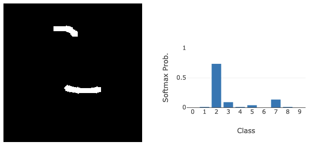
This work started as a curiosity about how AI/ML models perform classification, specifically, why they give the answers they do. As humans, we tend to anthropomorphise AI, which makes it surprising when we realise that it has no clue what it’s actually doing. An image classifier lacks semantic understanding of the images it’s classifying, which can lead to some really strange results (see below). By using explainability methods, we can see why a model assigns a class to an image. While most explanations make sense, they also help us create artificial inputs that have no semantic meaning to humans but still lead to highly confident responses from a model (see below).

Partway through this exploration, I thought, “Hey, allowing people to play with this would be cool!” So, this started the project.

I wanted people to be able to visit a web page, provide input to a classifier, and have the classification results returned to them along with an explanation of those results. From there, people could interpret the explanation and maybe use it to fool the model. In addition to providing a fun little website for people to play with, I’d gain experience deploying an AI/ML model in the real world, along with everything needed to make that a reality. What follows is an explanation of how this project works, the design decisions I made along the way, and what I learned in the process!

Project Outline

There are a few parts to this project. We need: 1) An MNIST classifier with explainability. 2) A way to interface with the MNIST classifier from a web page. 3) A way to publish the app so anyone can access it.

The MNIST classifier isn’t much of a problem. This will just be a small convolutional network built with PyTorch. We’ll train the model, store the weights, and then load it at runtime for inference. Since it’s just a small MNIST model, and the input will be a single $28 \times 28$ grayscale image, we don’t need to involve a GPU at inference time. The inclusion of Integrated Gradients for explainability shouldn’t add too much overhead either, so we should be fine with just CPU compute for this project. Of course, if we were handling large images, lots of inputs, or massive models, a GPU would be a necessity, but I’m being very cost-conscious here and don’t want to hammer in a nail with a sledgehammer. To include explainability with the classifications, I used Captum. A library that simply wraps the PyTorch model, and when given the image we’ve just classified, along with the prediction, it generates an explanation of how the model arrived at its classification. I decided to use the Integrated Gradients¹ approach to model explainability. To compute the integrated gradients of a model $F$ we start with the input to the model $x$ and a baseline $x’$. The baseline is essentially an input that should elicit no meaningful response from the network (i.e., a response as uniform as possible). In the case of images, this would be a black image. We select a dimension $i$ (a pixel in the case of images) and take a path integral of the gradient along a linear interpolation from $x$ to $x’$: \(IG_i(x) := (x_i - x_i') \cdot \int^1_{\alpha=0} \frac{\partial F (x' + \alpha (x-x'))}{\partial x_i} d\alpha\) Since $\alpha \in [0,1]$, we gradually move along the path from a completely black image to the original colour version. While this is happening, we’re paying close attention to the rate of change of the model output with respect to $x_i$. This allows us to understand the importance of dimension $i$ to the classification. Doing this for each pixel (or group of pixels) will enable us to see what parts of the input contribute most strongly to the output, producing a heatmap showing how each section contributes to the final class.

Interfacing with the MNIST classifier is an interesting part of this project for me. I’m a classically trained computer scientist, so most of the programs I’ve created in the past have been command-line only. This is often great for efficiency and getting to the core of the problem you’re solving, but it isn’t very accessible to the general public. Because I wanted this to be a web app to exercise my deployment muscle, I knew this would have to be a web page with some JavaScript to make it interactive. I could also use a Python backend to serve the web pages and interact with the model. This was the part I was most cautious about, 1) because I’ve not done much web programming before, and 2) because I’m a security person and know that there are a lot of things that can go wrong security-wise if you’re not careful with your web setup. This is the section I relied on LLMs most heavily. Using them to help me create the JavaScript for the frontend, plug it into the Python backend, and make sure I had addressed most of the obvious security issues. I can’t say the result is perfect, but it does work and I haven’t been hacked (yet, please don’t, if you do find any security issues, please tell me)!

To publish the app, I knew I wanted to use a popular service to gain experience on a well-known platform. I was using Docker for the entire project, so having some way to say: “here’s a Docker container, just make it work” was another aim. I settled on Google Cloud Run, which has the container approach I was looking for, integrated load balancing, good statistics tracking, and is free, provided I don’t exceed a set number of requests. I was a bit disappointed that I didn’t get to do much load balancing because it’s been a while since I’ve done any Kubernetes work, but Google Cloud Run just works, so maybe it’s a good thing not to have another point of failure that I’d have definitely messed up!

MNIST Classifier

Creating the MNIST classifier was fairly straightforward. I used a small architecture I’ve used for a few other projects, consisting of two convolutional layers and one fully connected layer before the output. Since MNIST is such a small dataset, I encountered overfitting issues, so I added some aggressive dropout after the convolution and fully connected layers with a probability of 0.5. The architecture could achieve good results on MNIST (>99%). After training the model weights were saved, and to reduce the project’s attack surface, I removed all training code, leaving only the minimal code to perform inference. The model is loaded and configured to evaluate inputs when the web app starts, so we only load it once per user. Explainability (provided by Captum) is implemented in the backend Python code after classification, with the Captum model initialised after the classifier is loaded from disk.

I admit that the architecture for the classifier is a bit more sophisticated than it needs to be, but I just grabbed a model that I’d previously used for CIFAR classification and wanted to make sure I didn’t run into any capacity issues.

The code for the classifier can be found here.

Real inputs are never simple

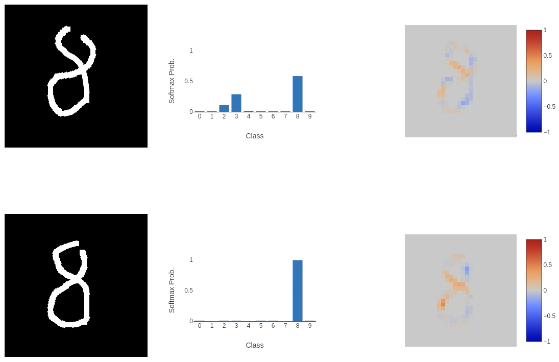
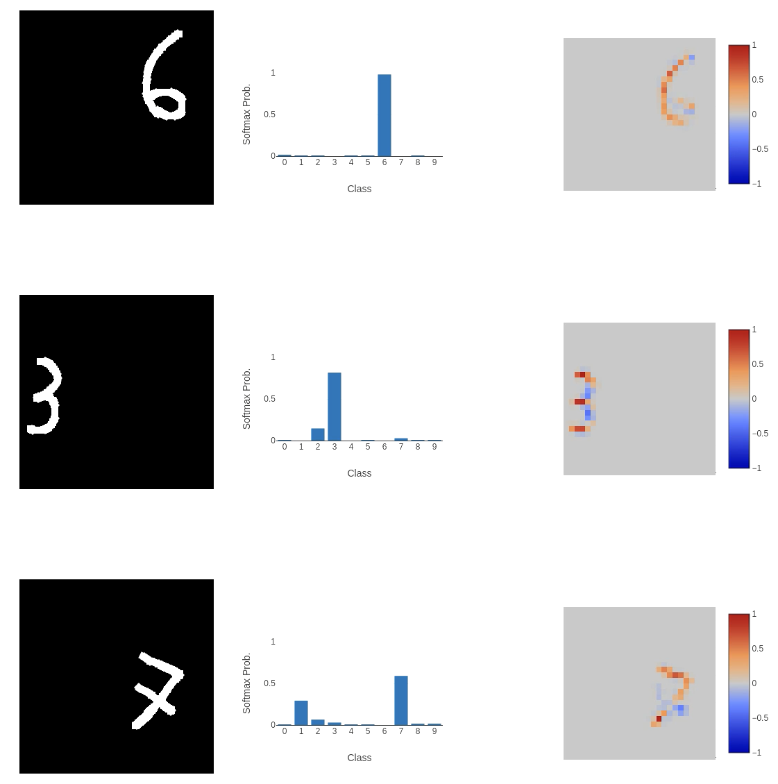
For this section I’ll skip forward a little, to after I implemented the interface. Once I had the web app code in place to provide input to the model, and a strong model trained (10 epochs, learning rate of 1e-4, final validation accuracy of 98.87%, loss of 0.0403, and 99.14% on the test set), I could finally test it end-to-end. 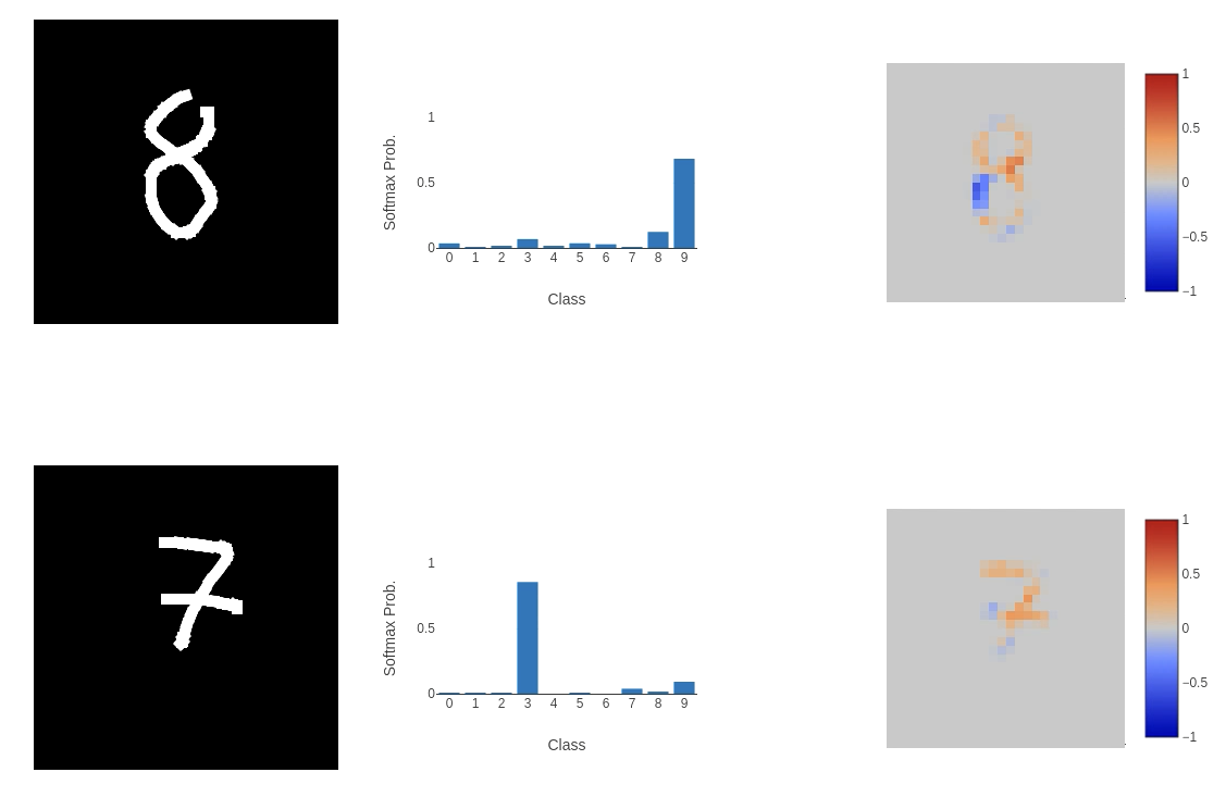This, unfortunately, didn’t go well. While the model performed as expected on some inputs, on others (as shown above), it failed to classify them correctly in highly perplexing ways. The integrated gradient explainability provides clues. The first image of the 8 (or 9 according to the model) places a negative weight on the bottom left curve of the input, meaning that it is not important to the classification process at all. A similar thing is happening in the bottom image: the left horizontal cross through the centre of the 7 and the line below it are being ignored. This does help to explain why the model is returning these classes (if we remove these sections of the input, we could argue that the 8 would look like a 9 and the 7 would be closest to a 3), but the question is: why is this happening?

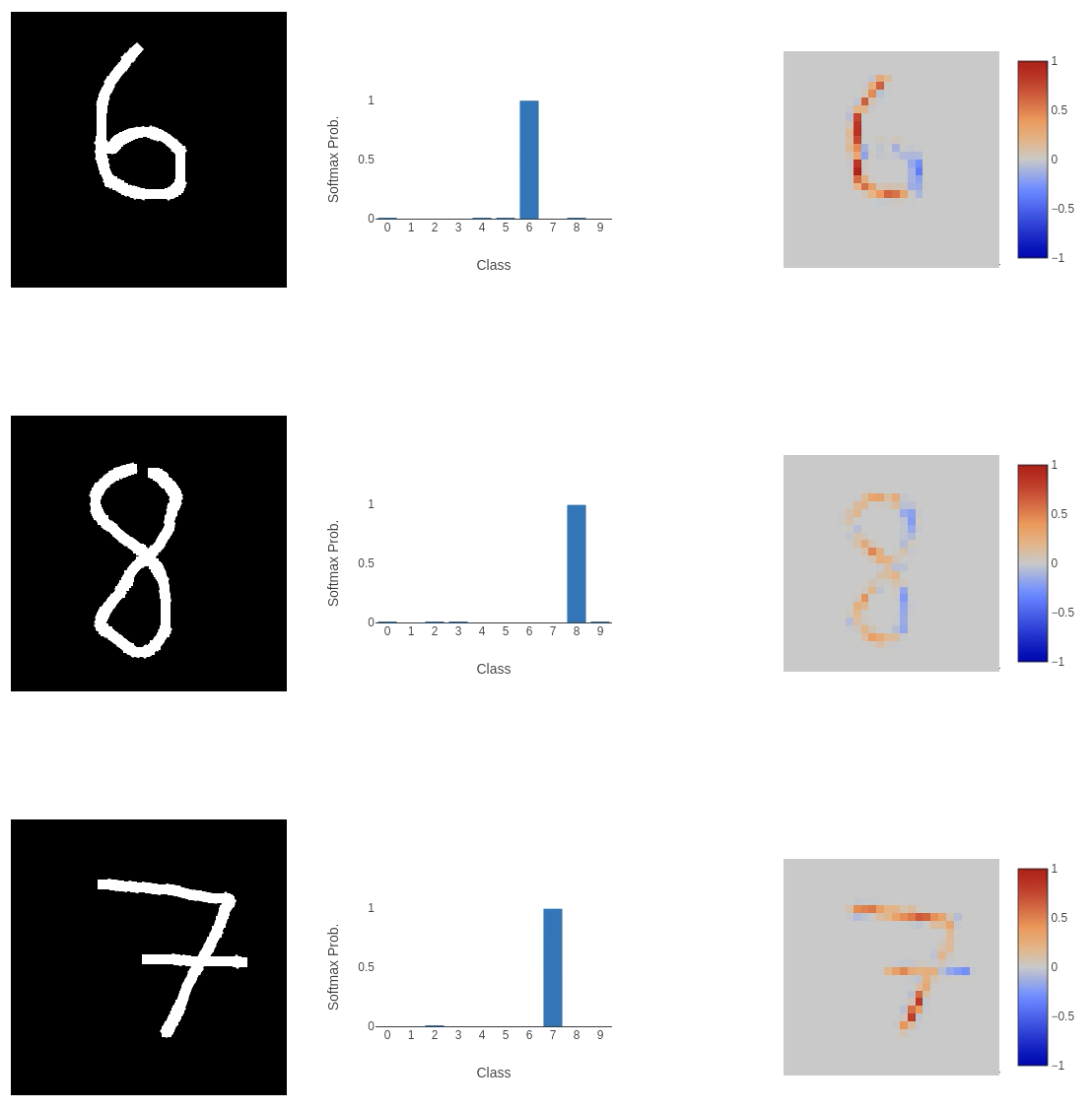
One argument I’ll address quickly is that the number of epochs is quite small. So let’s train longer (even though we achieve > 99% accuracy in just 10 epochs). Increasing the number of epochs to 25 (more epochs started to hint at overfitting), I achieved a validation set accuracy of 99.18%, with a loss of 0.0416, and a test set accuracy of 99.19%. 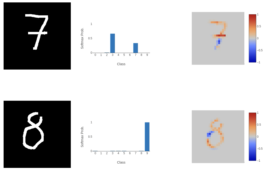Still not great! Although we do see greater confidence in attributing parts of the input to the classification.

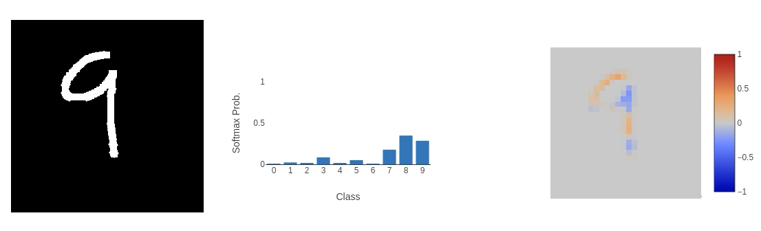
I thought the architecture might be too complex for such a simple task, so I removed the convolutional layers in favour of a simple fully connected network. This didn’t work out well. Even though this network is consistently the most confident, and the explanation is very clear where the classification comes from, it’s completely wrong!

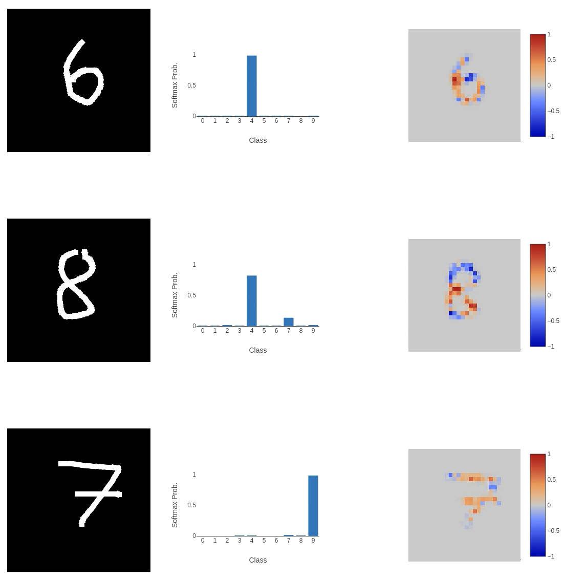
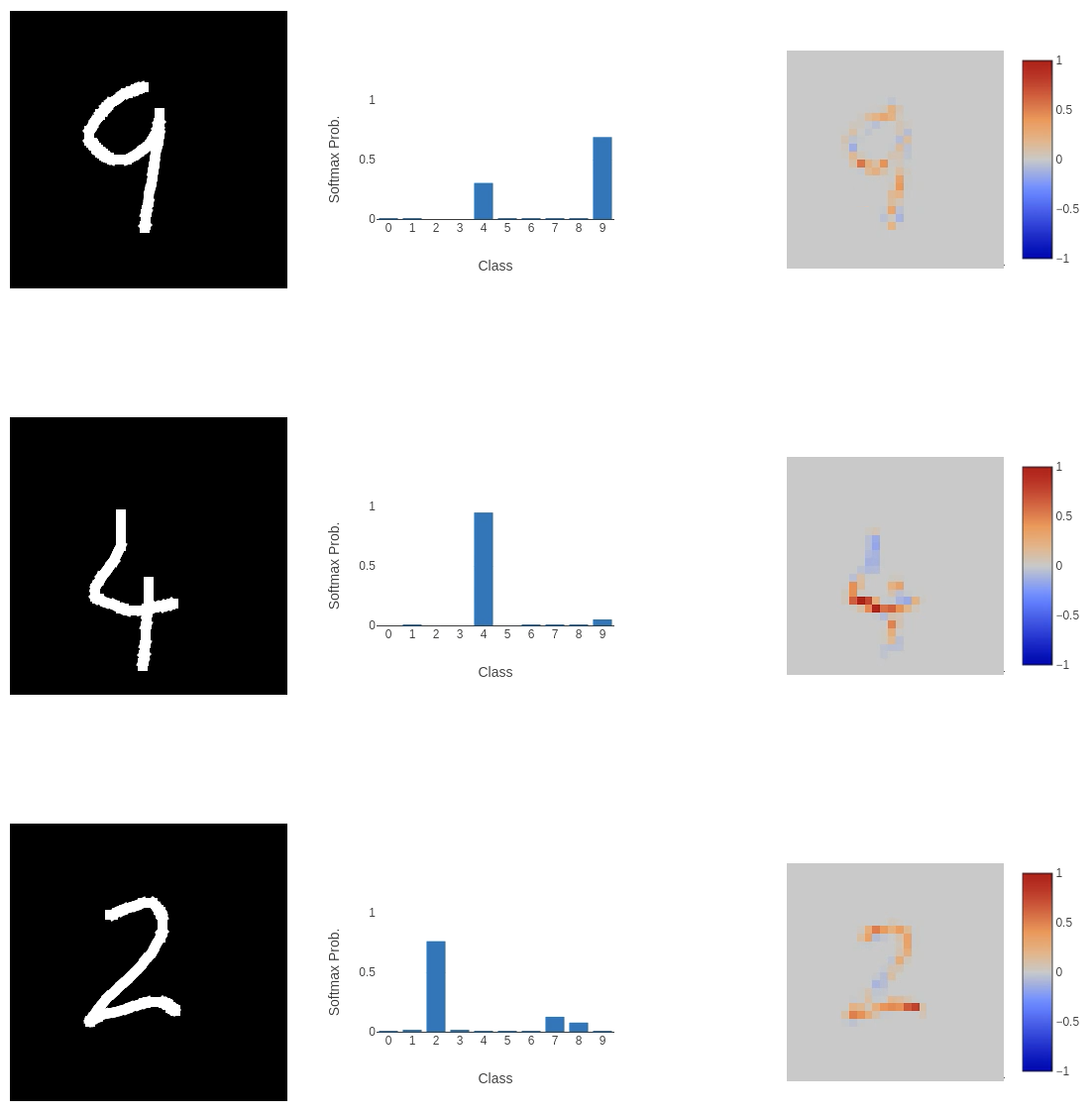
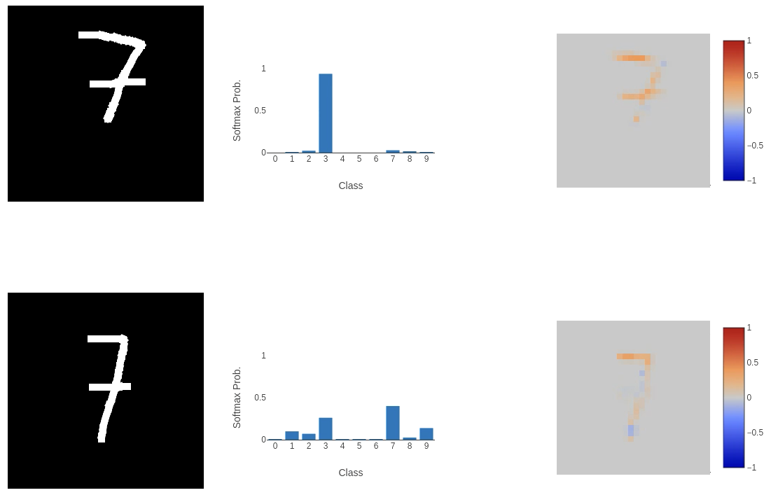
What if we revert to the original architecture and add dropout layers to regularise the model? The new model has a validation accuracy of 98.63%, a loss of 0.0498, and a test set accuracy of 98.73%. This seems to work quite well. But we also have some failures. The major departures in classification we see appear to come from inputs that don’t use the full space. For example, the first 7 in the images above. The MNIST dataset is a perfect encapsulation of the issue we run into when training models to perform a task and then send them out into the wild. That is: people provide weird inputs. 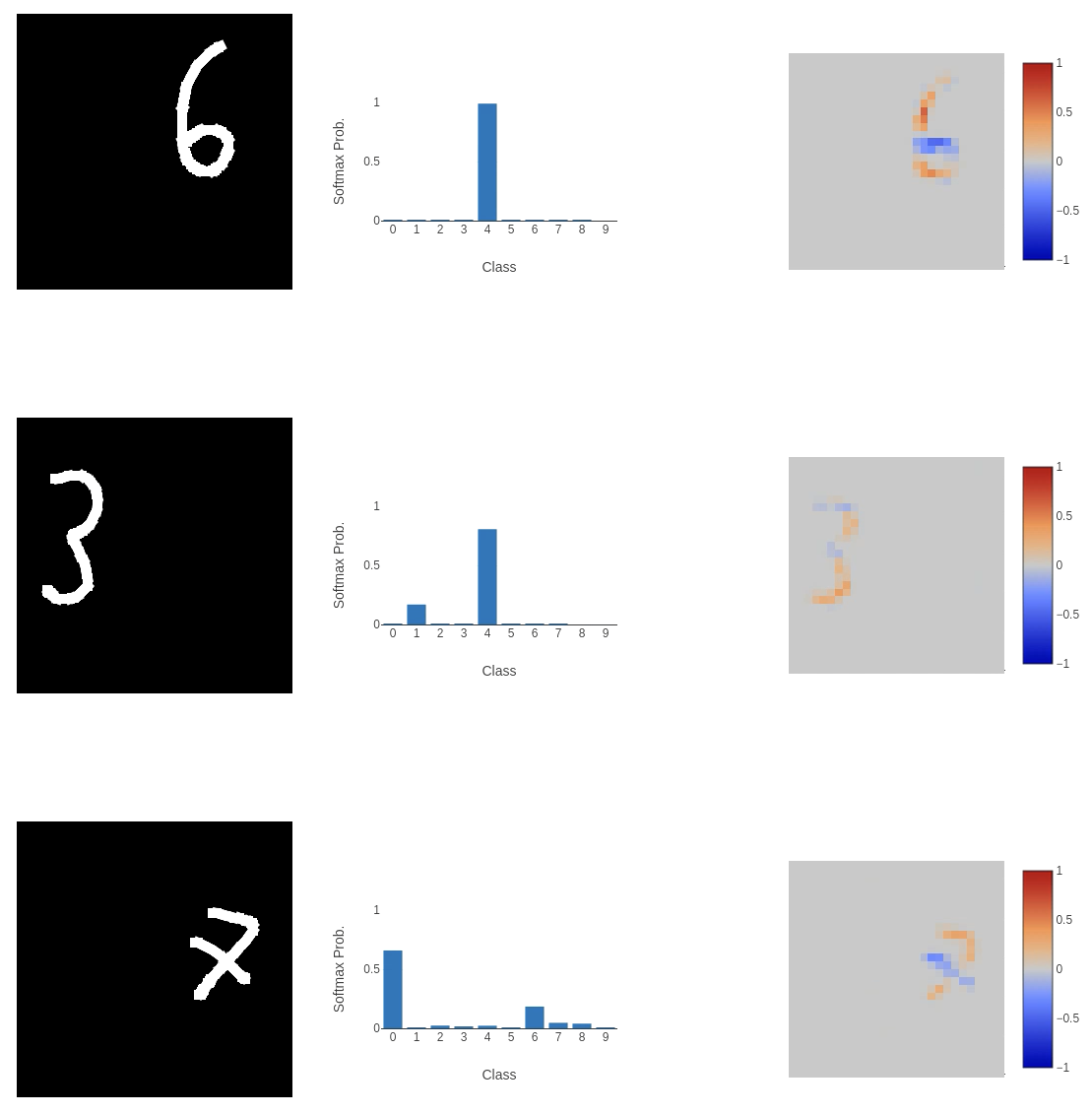7s are tiny, and on the right-hand side of the input space, 3s or 6s are squashed. We need to make the model more robust to the many ways people can squash their numbers into the input space, and the standard MNIST dataset doesn’t do this. The images are perfectly centred, scaled correctly and all straight. To allow the model to generalise to a wider range of inputs, we need to make the training dataset more varied.

Torchvision provides a really quick way to introduce the changes we want to make to the dataset. We use the RandomAffine transform:

torchvision.transforms.RandomAffine(degrees=30, translate=(0.4, 0.4), scale=(0.3, 1.7))

This function allows us to randomise the application of a variety of affine transforms, such as: Rotation (specified with the degrees parameter), which rotates the input by up to 30 degrees; Translation (translate parameter), which translates the input by a fraction of the size of the input horizontally or vertically (in this example, we translate the image by up to 40% of it’s size up, down, left, or right); Scale (scale parameter), which scales the image between 30-170% of its original size.

These transformations occur during dataset loading. This would be more effective if we applied them when passing the input to the model, but the results seem to work well enough without that extra layer of randomness in the training dataset!

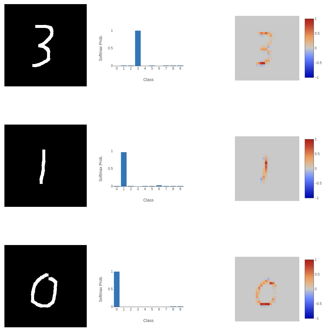
After training for 75 epochs, we have a validation accuracy of 80.05%, with a loss of 0.6576, and a testing set accuracy of 80.27%. While we do see a significant drop in the model’s accuracy, it is more robust to unexpected representations of valid inputs. And on the more general, centred inputs, we were struggling with before: Seems to work pretty well! This experience reminds me that you can never be too set in your ways when implementing any computer program or ML model that interfaces with a user. There’s always going to be something surprising that you never really considered. In this case, it was that the standard MNIST dataset is not very representative of the inputs you should expect from a user. Especially if you give them a lot of space to write in!

Building an interface

As I mentioned in the project overview, I didn’t have much experience creating frontends for web apps. I hadn’t really done much work with JavaScript, especially with interacting with users, sending information to a backend, and retrieving something to show on the page afterwards. Because of this, I relied on LLMs to help me get the code right.

I started by defining what the web app should do at a high level. I wanted a small black canvas that visitors could draw on with white ink (reminiscent of the MNIST dataset images). The user should then click a “Classify” button, and the MNIST model should classify the canvas content, returning the class probabilities along with an explanation heat map.

The drawing canvas wasn’t too difficult to get working because people have been drawing on web pages since the beginning of the internet, so a lot of functions already exist to make this easy. Something I hadn’t considered beforehand was adding touch drawing to make the app mobile-friendly. Adding touch drawing just involved a second drawing function, which wasn’t too much extra work. NOTE: The touch implementation is a bit buggy. I really need to look at that again. 😳 The model expects an input image of $28 \times 28$ pixels, but this is a bit small to draw on! To keep things easy to use and process, the drawing canvas is set to $280 \times 280$, and the image is scaled down by a factor of 10 before classification.

Sending the canvas content from the frontend to the backend is done through a POST request to the /classify endpoint in the FastAPI Python code. We pause (await) until we receive a JSON response that includes the classification labels, the softmax probabilities for each label, and the explanation heat map. This data is displayed using Plotly, clearly showing the input, prediction, and explanation for the prediction. All of this data is added to the top of the result stack, pushing all other previous classifications further down the page (I was probably more proud of making that stack work than I should have been!).

The code powering the front end can be found in the GitHub project, specifically here for the JavaScript and here for the HTML. I do not claim that it’s great JavaScript or HTML, but it works.

The backend, acting as a counterpart to the wonderful frontend, was written in Python using the FastAPI web framework. There’s nothing too interesting here. On startup, we load the classifier and create the integrated gradients model, both of which persist throughout the application’s lifetime. Classification happens at the /classify endpoint that takes the image as base64 data, converting it to an image using Pillow. As mentioned earlier, the classification is performed using the previously loaded classifier, with the softmax probabilities, labels, and the explanation heatmap image returned to the frontend.

An interesting part of the backend that I knew I needed to handle, but didn’t know how to approach, was the security of user input to the classifier. Any instance where user input interfaces with code is a security risk, so I wanted to make sure it was handled correctly. So, I asked Claude, which gave this response (imports included for clarity):

from pydantic import BaseModel, Field, field_validator
import base64
import io
from PIL import Image

class ImageRequest(BaseModel):
    image: str = Field(max_length=MAX_PAYLOAD_SIZE)

    @field_validator("image")
    @classmethod
    def validate_image(cls, input_data):
        # Check that it's a PNG data URL (reject anything that isn't)
        if not input_data.startswith("data:image/png;base64,"):
            raise ValueError("User input must be a PNG data URL")

        # First check passed! Next get the base64 data
        _, encoded = input_data.split(",", 1)

        # Validate that base64 is well formed
        try:
            binary_data = base64.b64decode(encoded, validate=True)
        except Exception:
            raise ValueError("Invalid base64 encoding")
        
        # Validate it's actually a PNG by checking for specific bytes
        if not binary_data.startswith(b'\x89PNG\r\n\x1a\n'):
            raise ValueError("Data is not a valid PNG")
        
        # Validate dimensions
        try:
            image = Image.open(io.BytesIO(binary_data))
            w, h = image.size
            if w != MAX_IMAGE_DIM or h != MAX_IMAGE_DIM:
                raise ValueError("Image dimensions exceed maximum size {}x{} > {}x{}".format(w, h, MAX_IMAGE_DIM, MAX_IMAGE_DIM))
            if w < 1 or h < 1:
                raise ValueError("Image too small")
        except ValueError:
            raise
        except Exception:
            raise ValueError("Could not parse image")

        return input_data

The star of the show here is Pydantic, which is a data validation library for Python. We define an ImageRequest class that inherits from BaseModel and has a single field: image. This starts as a string (it’s just a string of bytes), but we make sure that its size does not exceed MAX_PAYLOAD_SIZE, so we’re not ingesting an input that is larger than we expect, which could grind our poor cloud server to a halt (and quickly exceed our maximum memory capacity).

The validation of the input (the validate_image function, which has a decorator @field_validator("image") that I believe connects it to the class field) starts by ensuring the input data is labelled as a PNG. If this is true, the base64-encoded data is decoded into binary, with checks to ensure it’s correctly formatted (binary_data = base64.b64decode(encoded, validate=True)). But anyone can label any data as a PNG, so we have a check to ensure the first few bytes are consistent with the PNG file format (see the Magic number information in the summary thing on the right, which is consistent with the check: binary_data.startswith(b'\x89PNG\r\n\x1a\n')). Now that we know the file size is appropriate, it’s valid base64, and it’s actually a PNG, we can decode the bytes into an image, verify the image size matches what we’d expect, and then continue with classification.

The backend can be found in the main.py file here.

Publishing the app

To make publishing simple, portable, testable, updateable, etc. I Dockerised the program. I’ve been fairly comfortable with Docker for a while, so I knew it was the standard way to build apps that run on the internet. I did extend my knowledge with the build stages, though. As Claude pointed out, leaving all the installs I needed to install the Python libraries in the deployed container would create a larger attack surface than necessary. By building the libraries into a wheel file and passing it from the build to the runtime container, I could make the deployed container more secure and smaller. I also followed best practices to limit user permissions within the container (just in case someone broke out of the program), so that a potential adversary would not have superuser privileges.

The main application was served from the Docker container using Gunicorn, which has lots of options for the number of workers, timeouts, etc. This was bound to a port allowing the app to be served via the same exposed container port. The Dockerfile is here.

To deploy the Docker container, I used Google Cloud Run. This service had a number of attractive selling points, including: autoscaling - so the number of containers that are deployed can grow or shrink depending on demand (there won’t be much), it can automatically build containers from GitHub - so I can have continuous integration (CI) and continuous delivery/deployment (CD), and it handles the TLS/SSL certificate - so my app can use HTTPS. In addition, Cloud Run has access to GPU compute and large-scale storage (external volume mounting), should I ever need to expand the app with GPU-accelerated computing or massive datasets/models in the future.

I kept the setup fairly conservative because this is just a test app, and I don’t expect it to be a massive service that gets lots of traffic:

• I set the minimum number of instances to 0, so if the app doesn’t need to run, it won’t! This also cuts down on costs because I won’t have a container constantly running just in case someone visits. I’m not too worried about cold starts. It does take a bit of time for the app to load sometimes, but that’s a trade-off I’m willing to make.
• The maximum number of instances is 3. I don’t expect many people to access this at once, or at all, so keeping the maximum number low lets me control costs better and make sure expenses don’t get out of hand.
• I gave each instance 512 MiB of memory, and from the service metrics, container memory utilisation is around 80%, so this was a good call! It’s nice to see there’s not much wastage there.
• Each instance has 1 virtual CPU because it doesn’t really need much more. It’s fairly lightweight and performs well.

For the CI/CD portion of this project, I hooked up my GitHub repo to the cloud service to automate the development and deployment process. Cloud Run allows you to add triggers, so when new data is pushed to the repo the Docker container is automatically built, checked and deployed to the service, which streamlines the workflow massively.

Conclusion

So, I have a web app now! You can check it out at letsfoolai.cloud. You can read a bit about how to fool a classifier and then try it out yourself! I don’t expect this to be a very popular app (it’s not that interesting), but I’m so happy it all came together, and it works!

This has been such a learning experience. From the classifier to the web server to the deployment, I’ve had to force myself out of my programming comfort zone to do something new. It’s been a headache at times, primarily in deployment, because that is something that I have no experience with, and understanding all the steps I had to go through to deploy containers and then bug fix what went wrong with very in-depth service analysis pages (I had issues with log file permissions, errors in container deployment due to too little memory, etc.). It has been tough, but so worthwhile! At least now I have a small idea about how modern applications are made available to the masses, and I will sympathise with the engineers if a well-known service is down. 😆

---

References

1. Axiomatic Attribution for Deep Networks - Sundararajan, Taly, Yan (2017) ↩