Natural adversaries and out-of-distribution detection
The research space of adversarial examples is one which is quite counterintuitive (we can easily change the result of a classifier by making invisible changes to an image) so I’m always looking for nice ways to conceptualise what’s going on. I encountered a nice explanation of a potential feature of adversarial examples in a paper by Smith et al. [1]:
Such examples lie off the manifold of natural examples, occupying regions where the model makes unconstrained extrapolations.
This statement (if accurate) is a really interesting one if we want to try and detect adversarial examples. We would be able to add an Out-of-Distribution (OoD) detection step to our system which will flag inputs which lie off the manifold of natural data either because the network was not trained to handle that input data, or because we’ve encountered an adversary (both of which are situations where we should ignore the predicted class). The idea behind OoD is that if we train a Deep Neural Network (DNN) to perform a particular task such as classification we need to provide the DNN with data and the corresponding labels of that data. During the training process we pass this data to the DNN and it builds a mapping from an input space to an output space. This input space has a particular geometry to it (approaching this from a probabilistic stand-point, the input data follows a distribution) which we can learn. If we have an input provided to us which is far away from this input geometry we’ve created (it does not belong to the same distribution) then if we can detect this, we can return an error or some warning of uncertainty around the results we provide.
A common method of OoD detection is a Bayesian Neural Network (BNN) which is similar to a standard DNN except we place distributions over the weights and biases meaning the network is no longer deterministic. To detect OoD data we can query the BNN with the same example multiple times and determine the deviation of results. The amount of devation gives us an idea around the uncertainty of the BNN in the classifications and can act as a proxy for the OoD methods. This is a very popular approach to OoD detection and has shown some good results in detecting adversarial examples in Smith et al. [1].
This concept of OoD detection pairs nicely with a second paper I found which presents “Natural Adversaries” by Zhao et al. [2]. Natural Adversaries (NAs) aim to create adversarial examples which are more natural to humans. Usually standard attacks such as FGSM [3] or Carlini & Wagner (CW) [4] create adversaries which have an unnatural perturbation. The pixels that are altered can be from any part of the image which often leads to noticeable patterns emerging, or sharp changes in pixel values. The approach NAs take is to make semantic perturbations which appear more natural (e.g. increasing the thickness of a particular line in the image). An example can be seen in the image below which shows that the perturbation is localised to salient parts of the image.
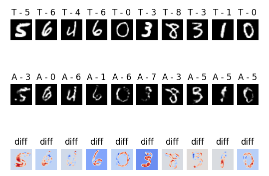
The image below shows the difference between the perturbations of all of the adversarial attacks which hilights the focus of NAs on the important parts of the image.
Due to the proposed naturalness of the image, a question we can ask is:
Is a Natural Adversary out-of-distribution?
This forms the first part of this exploration.
Are Natural Adversaries OoD?
First, we need to discuss the process of generating NAs (which also raises a host of other interesting questions, but one at a time).
Generating NAs
The NA method is a black-box adversarial generation method (it does not require any access to target model internals, such as weights, biases, training method etc.). All we need is to know what task it performs (which is fairly easy if you have a working system “in the wild”) and then create a dataset which we imagine would be effective at training the model to do that particular job.
As usual, we have a target (black-box) classifier $f$ we want to fool and a dataset $X$ of unlabelled data. The goal is to generate an adversarial input $x^ * $ from a clean image $x$ which causes a misclassification $f(x) \neq f(x^ * )$. In practice it is not necessary that $x \in X$ since this is not the case for inputs when the model is deployed, but we do assume that the we’re working with some underlying distribution $\mathcal{P}_x$ that $x$ is sampled from ($x \sim \mathcal{P}_x$). The key part of producing natural adversaries is that we want $x^ * $ to be as close to $x$ as possible in terms of the manifold that defines the data distribution $\mathcal{P}_x$ rather than the original data representation. This also avoids dodgy metrics that are often associated with image similarity, such as $L_2$-norms.
Traditional approaches to adversarial attacks focus on searching for adversaries directly in the input space. Zhao’s method searches in a corresponding dense representation of $z$ space. Therefore, rather than finding an adversary in the input space (giving us $x^ * $ directly) an adversarial $z^ * $ is found in an underlying dense vector space which defines the distribution $\mathcal{P}_x$. This is then mapped back to an image $x^ * $ with a generative model. By using the latent low-dimensional $z$ space adversaries are encouraged to be valid and semantically close to the original image since it is close to the underlying distribution.
Powerful generative models are required to learn a mapping from a latent low-dimensional representation to the distribution $\mathcal{P}_ x$ which is estimated using samples from $X$. Using a large amount of unlabelled data from $X$ as training data, a generator $\mathcal{G}_ \theta$ learns to map noise with distribution $p_z(z)$ (where $z \in \mathbb{R}^d$) to synthetic data which is as close to the training data as possible. A critic $\mathcal{C}_ {\omega}$ is also trained to discriminate the output of $\mathcal{G}_ \theta$ from the true data of $X$.
The objective function for this GAN (refined using the Wasserstein-1 distance making it a WGAN) is defined as:
\[\underset{\theta}{\text{min}}\; \underset{\omega}{\text{max}} \; \mathbb{E}_{x \sim p_x(x)}[\mathcal{C}_ \omega(x)] - \mathbb{E}_{z \sim p_z(z)}[\mathcal{C}_ \omega(\mathcal{G}_ \theta(z))]\]To represent natural instances of the domain a WGAN is trained on a dataset $X$ which gives us a generator $\mathcal{G}_ \theta$ which maps random dense vectors $x \in \mathbb{R}^d$ to samples $x$ from domain $X$. A matching inverter $\mathcal{I}_ \gamma$ is used to map data instances to corresponding dense representations. We can informally think of these as $\mathcal{G}_ \theta : Z \to X$ and $\mathcal{I}_ \gamma : X \to Z$ where $X$ is the input space and $Z$ is the latent space. The reconstruction error of $x$ is minimised and we also minimise the divergence between sampled $z$ and $\mathcal{I}_ \gamma(\mathcal{G}_ \theta(z))$ to encourage the latent space to be normally distributed. This is described with the following equation:
\[\underset{\gamma}{\text{min}}\; \mathbb{E}_{x \sim p_x(x)} \| \mathcal{G}_ \theta(\mathcal{I}_ \gamma(x))-x \| + \lambda \cdot \mathbb{E}_{z \sim p_z(z)}[\mathcal{L}(z, \mathcal{I}_ \gamma(\mathcal{G}_ \theta(z)))]\]For images, the divergence $\mathcal{L}$ is the $L_2$-norm, and the constant $\lambda$ is set to 0.1. The aim here is to change $\gamma$ to minimise the sum of the expected values. The first part ($\mathbb{E}_ {x \sim p_x(x)} | \mathcal{G}_ \theta(\mathcal{I}_ \gamma(x))-x |$) is the difference between the input $x$ projected to the latent space, then projected back to the input space, and the actual input. The second part ($\lambda \cdot \mathbb{E}_ {z \sim p_z(z)}[\mathcal{L}(z, \mathcal{I}_ \gamma(\mathcal{G}_ \theta(z)))]$) is the weighted expectation of the divergence between a point in the latent space and the result of projecting that point to the input space, then back to the latent space. In essence, we’re minimising the differences between the two projection directions.
With the learned functions $\mathcal{I}_ \gamma$ and $\mathcal{G}_ \theta$ a natural adversarial example $x^ * $ is defined as:
\[x^ * = \mathcal{G}_ \theta(z^ * ) \text{ where } z^ * = \underset{\tilde{z}}{\text{argmin}}\; \| \tilde{z} - \mathcal{I}_ \gamma(x) \| \text{ s.t. } f(\mathcal{G}_ \theta(\tilde{z})) \neq f(x)\]The difference with traditional adversarial generation techniques is that for this method, the perturbation is performed in the latent space of the input, then projected back into the input space to check if it successfully fools the classifier.
A step-by-step guide:
-
Project the input into the latent space: $z’ = \mathcal{I}_ \gamma (x)$
-
Apply perturbations to $z’$ giving us $\tilde{z}$ which aims to generate an adversarial result
-
Project the perturbed $\tilde{z}$ onto the input space: $\tilde{x} = \mathcal{G}_ \theta(\tilde{z})$
-
Check if it fools the classifier: $f(\tilde{x})$
OoD Detection using BNNs
BNNs allow us to analyse two different types of uncertainty in classification, epistemic (uncertainty because of a lack of knowledge) and aleatoric (uncertainty because of natural noise in the data). For OoD detection we’re more concerned with epistemic uncertainty which can act as a proxy for the distance to the natural data manifold. Since epistemic uncertainty is focused on the information the model does not know, we can easily see that since the natural data manifold is built from the information the model is trained on (and therefore has knowledge of) the epistemic uncertainty can be used for OoD detection.
The two measures used for epistemic uncertainty are Mutual Information (MI) and Softmax Variance (SMV). Both can be used as a proxy for the distance from the natural data manifold. The details of these particular measures can be seen in [1]. I won’t go into them here since they get a bit technical, but all we need to know is that higher MI and SMV mean images are further OoD.
Are NAs OoD?
Since the generated adversaries aim to be as close to the natural distribution as possible it’s interesting to consider whether or not NAs are OoD or not. From some experimentation I’ve carried out, it appears not (see the tables below). We pass a clean set of images to a BNN followed by the set of images after having an FGSM attack applied to them, then C&W then finally the NA attack. The MI and SMV was calculated for the results of 100 queries of the BNN.
| Clean | FGSM | C&W | NA | |
|---|---|---|---|---|
| Accuracy | 98.0% | 9.0% | 5.0% | 5.0% |
| Clean | FGSM | C&W | NA | |
|---|---|---|---|---|
| Mean MI | 0.0245 | 0.0972 | 0.0385 | 0.203 |
| Mean SMV | 6.80e-4 | 3.09e-3 | 1.00e-3 | 6.41e-3 |
| Relative MI | 0.695 | 2.76 | 1.09 | 5.76 |
| Relative SMV | 0.670 | 3.04 | 0.983 | 6.31 |
This table shows the mean MI and SMV for a number of different adversarial attacks and clean images. Also included is the relative MI and SMV using a seperate set of clean images as a baseline. This shows that the MI and SMV of the NA method is far higher than the other adversarial attacks (even over FGSM) which indicates that this method isn’t particularly effective at creating adversaries which remain in distribution.
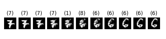
The reason for this could be that, when we create a NA we’re using a continuous dense vector space to produce the perturbation (which can be seen through the images of interpolation between two classes, see image below). The image actually starts to look more like the class we target since we can only change the semantic parts of the image. This means that when we apply a perturbation we’re naturally going to be somewhere in between classes which could cause the increased uncertainty which leads to the OoD detection by BNNs.
Correcting Adversaries
The architecture of the NA method is an interesting one. We have created a GAN which allows us to map from an input space to a dense vector space and back again. Can we do anything else with it? We can reconstruct images fairly well and if we take a random vector from the embedding space and map it to the input space we end up with nothing recognisable (which means we have a well defined space, see image below) so what happens if we feed adversaries into it? Can we avoid adversarial attacks by passing them through the GAN, get a reconstruction and perform the classification on that reconstruction?
The next question is:
Can we use the architecture of the NA to correct adversaries?
We start by creating a number of perturbed images (1000) using FGSM and C&W then for each of the images in these sets we map them to the dense vector space then back again. The results are in the table below.
| Clean | FGSM | C&W | Clean Reconstructed | FGSM Reconstructed | C&W Reconstructed | |
|---|---|---|---|---|---|---|
| Accuracy | 97.0% | 11.0% | 2.00% | 94.0% | 79.0% | 93.0% |
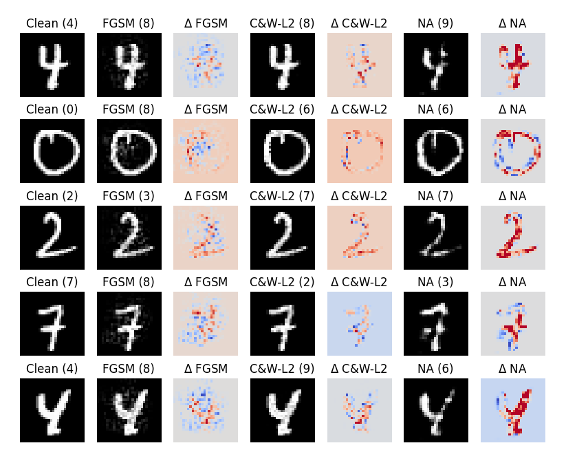
If we look at the FGSM results, we can see that the reconstruction method improves the accuracy of the model by approximately 60% which is a huge improvement. Even more suprisingly, the more advanced C&W attack sees an increase in over 80% accuracy which is a massive gain. Examples of the clean images, adversaries and the reconstructions can be seen in the image below.
I found the results in the table above quite suprising. FGSM is the simpler adversarial attack which applies more obvious perturbations to an image than C&W, so why is the reconstruction accuracy of FGSM considerably lower than C&W? I think the answer can be found by looking back to the OoD tests we performed. The MI and SMV of C&W was much less than that of FGSM which means it is closer to the natural data manifold. This means that when reconstructing C&W images they’re closer to the natural manifold and their original position on it which is likely to be close to the true class which results in smaller adversarial perturbation and an easier reconstruction (projection back to the natural manifold). On the other hand, FGSM has a higher MI and SMV which means it’s further from the natural data manifold and so projection back to the manifold may result in the image being in a different classification region anyway. Evidence for this can be seen in the image above which shows that the reconstructed image does not necessarily have the same class as the original adversary.
This is backed up by further results which include adversaries generated by the NA method which lie far from the natural data manifold, therefore, further OoD.
| Clean | NA | NA Reconstructed | |
|---|---|---|---|
| Accuracy | 97.0% | 3.0% | 27.0% |
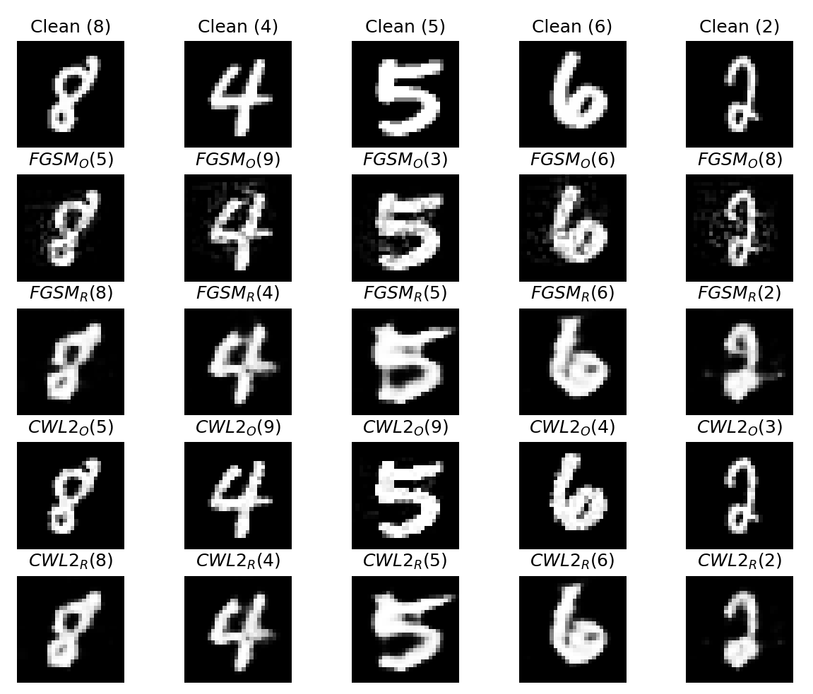
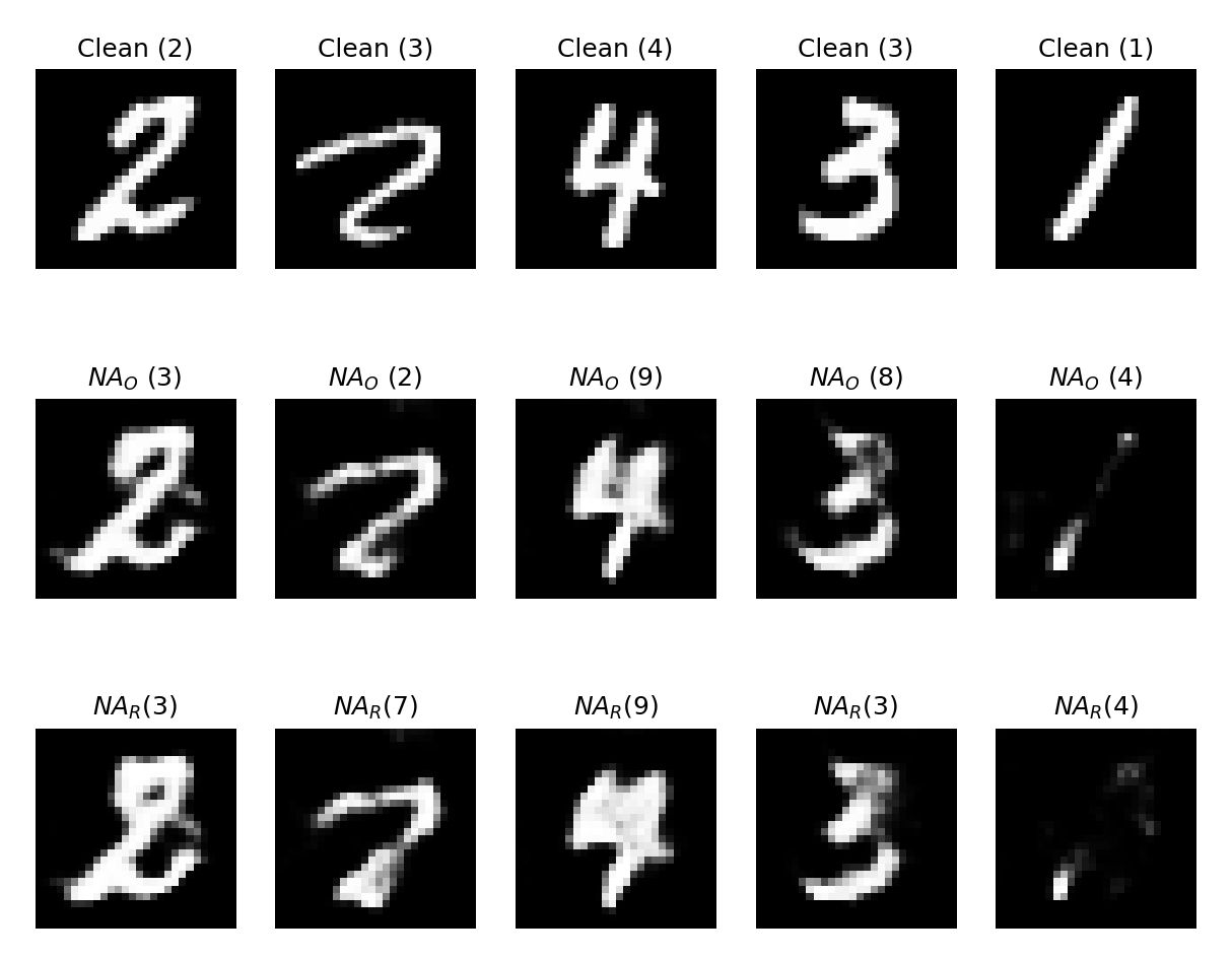
This result shows that the reconstruction of NA perturbed images leads to a small improvement, but nothing close to the improvements seen from FGSM or C&W which indicates that the further OoD an image is, the more difficult it is to correct using reconstruction methods. Essentially the perturbed image is so far from the natural data manifold it is a challenge to map it back correctly! Examples of these reconstructions can be seen below.
[1] Smith L, Gal Y (2018) - Understanding Measures of Uncertainty for Adversarial Example Detection
[2] Zhao Z, Dua D, Singh S (2017) - Generating Natural Adversarial Examples
[3] Goodfellow I, Shlens J, Szegedy C (2015) - Explaining and Harnessing Adversarial Examples
[4] Carlini N, Wagner D (2017) - Towards Evaluating the Robustness of Neural Networks