Explainable AI

Introduction

Machine Learning and AI models are often viewed as closed-box systems where we provide input and receive an output, and we don’t have a clear idea of how a model arrives at its answer. This lack of transparency can be unnerving depending on the context in which the model is being used, for instance, in safety- and security-critical systems or where major decisions are being made (deciding whether to accept a loan application, etc.). In addition, sometimes it’s just nice to see that a model understands the problem you have assigned to it and is not using some underlying unrelated aspect of the training data to find a shortcut to an answer (leading to failures when deployed in the real world).

Explainable AI methods focus on attributing the prediction of a DNN to input features. In the case of image classification networks, attribution can be assigned to patches of an image (see occlusion attribution) or even down to the pixel level (see integrated gradients).

I have personally used this approach to discuss the effectiveness of models with collaborators, highlighting how datasets are lacking, or questioning the bounds of the task the AI/ML model is required to perform.

Occlusion Attribution

Occlusion-based attribution¹ is the simplest approach to explainable AI for vision models. With this method, we pass an input to the model and record the output. We then occlude a part of the image by adding a black rectangle of a chosen size and then pass the new input to the network, measuring the change between the original output value and the new one. This rectangle is passed over the image (similar to a convolution kernel). By comparing the change in the output values at the different positions of the occluding rectangle, we can determine the importance of parts of the image to the result. The attribution can be represented as a heat map, which leads to a nice visual way of exploring this aspect of models.

Integrated Gradients

Integrated Gradients² were developed by Sundararajan, Taly & Yan in 2017 to address some of the shortcomings of other explainable AI methods, such as Occlusion-based attribution and DeepLift³. The authors posit that two axioms are important when attributing features to a network output. These are:

1. Sensitivity
2. Implementation Invariance

We’ll dive a little more into what these actually mean:

1) Sensitivity - Says that if we pass an input feature and a baseline (a black image in the case of a vision model or the zero embedding vector for text models) to a model, and they produce different outputs, then a non-zero attribution should be assigned to the input feature.

2) Implementation Invariance - The attributions assigned to two functionally equivalent models (models where the input-output pairings are identical, but implementations differ) should be the same.

While I find the sensitivity argument intuitive to understand, I struggle a bit more with the implementation invariance. The authors argue that during backpropagation of the output with respect to the input, the gradients of the model internals get cancelled out, leading to invariance. This makes sense, but it makes me wonder how true this is in practice. The authors state that if an attribution method fails to be implementation invariant, then the attributions may be sensitive to unimportant aspects of the models, e.g. if the model has more degrees of freedom than necessary to represent the function. From my understanding, model capacity (somewhat related to degrees of freedom) is an incredibly difficult metric to capture (and in my experience, models tend to have higher capacity than needed), so to state that implementation invariance relies on this makes me somewhat confused (but as always, I’m quite sure I’ve probably missed a part of the argument!). If models have more degrees of freedom, this means that a change to the output can be attributed to more than one input feature; therefore, two functionally equivalent models can choose to optimise different features to perform their task, leading to functional equivalence, but not implementation invariance (according to the paper).

To compute the Integrated Gradients of a model $F$, the authors start with an input $x$, and baseline $x’$ and select a dimension $i$ (a pixel in the case of images, or a specific feature like number of bedrooms or square footage in the case of tabular information). A path integral of the gradients is then taken along a linear interpolation from $x’$ to $x$. This is summarised as:

\[\text{IG}_ i(x) := (x_ i - x'_ i) \cdot \int^1_ {\alpha=0} \frac{\partial F(x' + \alpha(x-x'))}{\partial x_ i} \; \text{d}\alpha\]

The value of $\alpha$ is defined as $\alpha \in [0,1]$, which gradually moves along the path towards the original image $x$.

An added advantage of Integrated Gradients is that unlike Occlusion Attribution, the input images are not changed in a way that can lead to unnatural images (images outside of the distribution the models have been trained to operate on). For Occlusion Attribution, any changes in classification assigned to areas of an image could be due to the out-of-distribution nature of the images instead, causing inflated importance of certain parts of the image.

Attribution in Practice

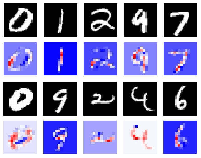
If we start with a simple MNIST model (two convolution and a fully connected layer, trained to 99% test accuracy), we can see the Occlusion and Integrated Gradients attribution methods in practice.

These are the results for the Occlusion attribution (red indicates positive attribution to the class):

These are the results for the Integrated Gradients attribution:

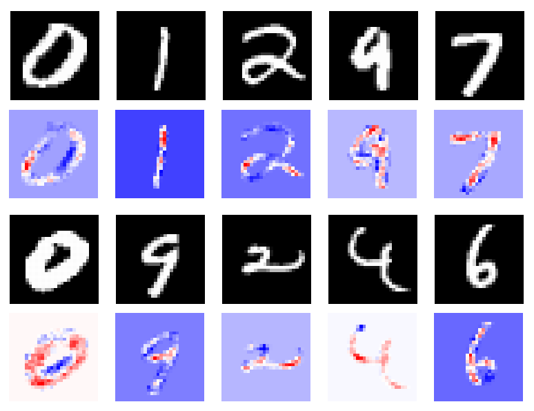
As we can see these two sets of results are very similar, with the Integrated Gradient approach having slightly more detail in the attribution. We could probably reduce the stride and sliding window shape further for Occlusion attribution to match the detail of the Integrated Gradients, but this starts to defeat the object of occluding blocks of the image (we’d essentially just be turning individual pixels off at that point).

From this we can start to infer some interesting behaviours of the network we’re analysing:

• First, a zero does not need to be a fully enclosed circle (some gaps are allowed), which makes sense since some people do not draw a fully enclosed circle, with the lack of completion occurring at any degree of the circle! It’s interesting to see that this is being taken into account.
• Second, the number 2 (fitting for the second example) is identified if there is a curved horizontal line, with a slanted line emerging from the (approximate) centre of it.
• Finally, the vertical (ish) line of the number 9 has questionable importance during classification. Provided we have a concave curve at the top of the image and some form of mark below it closer to the bottom of the image, it’s quite happy to consider that a 9!

From these findings, we can do some exploitation of the model! See the results below for examples of this.

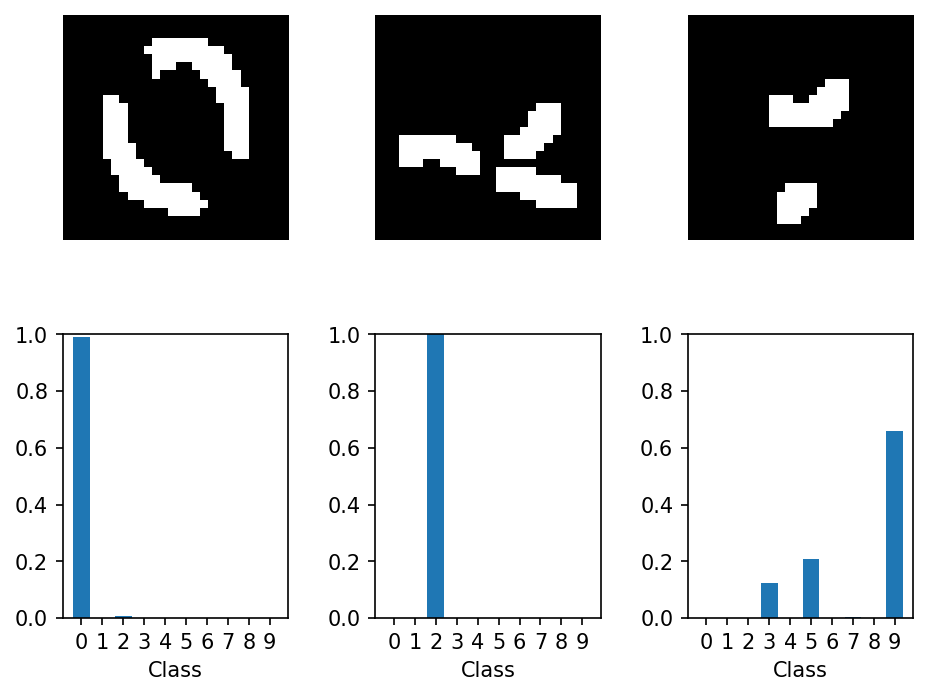
These images show that we can take the information we discovered about the attribution of features to classes and create examples which have no semantic meaning, but result in high-confidence classifications. The image of the ‘2’ here is particularly striking in just how devoid it is of meaning, yet the model is 100% certain that it’s a 2. This reminds me of rubbish images, discussed in a previous post! From these images, we can find weaknesses in datasets which we may be able to address with more data, correcting the ‘holes’, or we may even discover an edge case in the problem we’re trying to solve. All of which leads to interesting conversations and a more exact definition of the task the AI should perform!

Applying attribution to larger models (Inception V3⁴) pre-trained on the ImageNet dataset, we see similar attribution areas in Bronco the beagle⁵.

Occlusion attribution:

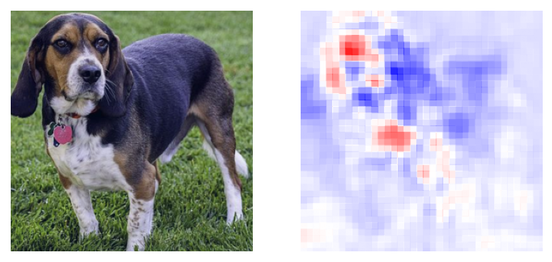
Integrated Gradients:

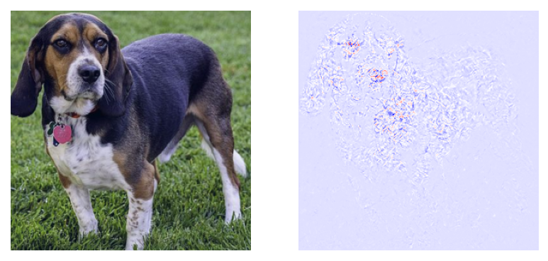
Both Occlusion and Integrated Gradient attribution highlight the nose, left eye and part of the shoulder as areas that contribute strongly to the classification!

Conclusion

Hopefully this exploration has been interesting! Explainable AI methods provide a really nice visual way to describe what models find important in the classifications they return. From this we can understand where failure modes may exist in underperforming models and address them, either through training on edge cases or a respecification of the task they are being asked to perform.

---

1. Zeiler and Fergus (2013) Visualizing and Understanding Convolutional Networks ↩

2. Sundararajan, Taly & Yan (2017) Axiomatic Attribution for Deep Networks ↩

3. Shrikumar et al. (2019) Learning Important Features Through Propagating Activation Differences ↩

4. Szegedy et al. (2015) Rethinking the Inception Architecture for Computer Vision ↩

5. Bronco the Beagle, PumpkinSky, CC BY-SA 4.0 https://creativecommons.org/licenses/by-sa/4.0, via Wikimedia Commons ↩