Feature Visualisation Part 3 - Update
Since the last network visualisation post, I have spent time refining and perfecting the approach to producing the best images using the most straightforward code! This is partly because it forms part of my thesis and partly because I like to explore the internal representations of Convolution Neural Networks (CNNs).
In the previous post on visualisation, I highlighted Total Variation and Diversity as two losses we need to account for when producing images that maximally activate a kernel. It turns out that this isn’t really necessary, and we can produce images that are just as good by using transformation (translations, rotations and scaling) between rounds of optimisation. This was the first simplification. The second was that we sometimes had non-convergence in some of the images (they remained grey), which could have been due to the lack of ReLU redirection. ReLU redirection is necessary during early rounds of optimisation since the target kernel may not be active; therefore, no optimisation can be performed, leading to non-convergence (see this python file for more information). In addition, because the original code (Lucid and Lucent) used gradient descent rather than ascent (and the whole idea is to maximise the activation), there were some extra steps necessary to make sure the gradients were being traversed in the correct directions. To simplify this, I’ve changed the optimisation to focus on maximisation:
opt = torch.optim.Adam(params=[image_c.spectrum_mp], lr=lr, maximize=True)
and added a small amount of noise to the gradients to kickstart image generation if there are no gradients to follow:
def image_grad_hook(grad):
    grad = grad / (torch.norm(grad) + 1e-8)  # Normalizing to unit norm
    grad = grad + torch.normal(mean=0, std=1e-6, size=grad.shape).to(device)
    return grad
Apart from these changes, nearly everything is the same! Through testing, it also achieves results that are pretty close to Lucent, all within 330 lines of code!
While the code is specifically designed to work with GoogLeNet1 (it uses the TorchVision GoogLeNet transforms, and the undo_decorrelate function uses the colour correlation matrix specifically calculated for GoogLeNet), it seems to work really well for ResNet2!
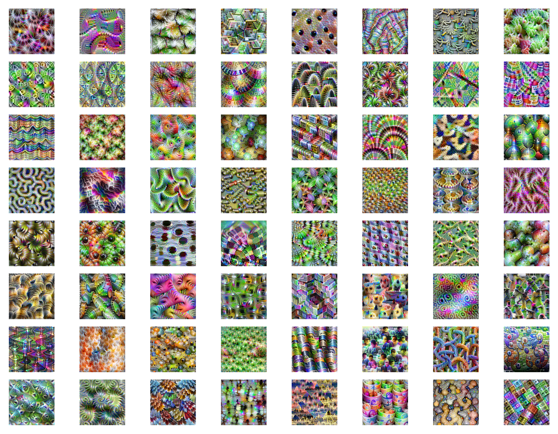
The images are included below, starting with the GoogLeNet activation images from 4c.branch4.1.conv:

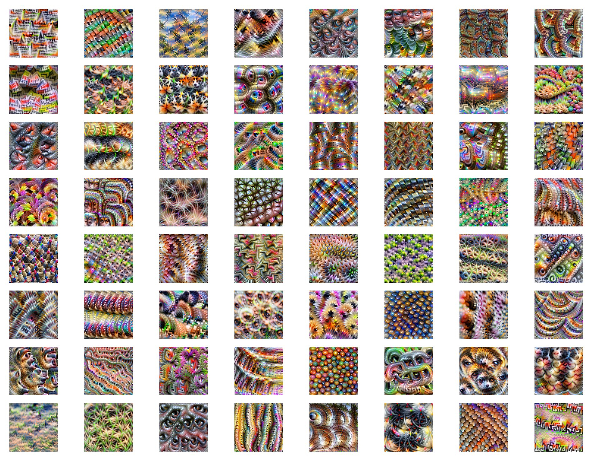
These are the activation images from ResNet-18 layer3.1.conv2:

The full code to produce these visualisations is here:
# BatchNorm based visualisation!
import torch
import torchvision
from torchvision.transforms import v2
import numpy as np


class Activation(torch.nn.Module):
    """
    Define a new loss function for visualisation
    """
    def forward(self, activation):
        """
        Overrides the default forward behaviour of torch.nn.Module

        Parameters:
        - activation (torch.Tensor): The activation tensor after the network function has been applied to the image

        Returns:
        - (torch.Tensor): The mean of the activation tensor (avoiding the boarder to reduce artifacts)
        """
        filter_act = activation
        # filter_act = activation[2:-2, 2:-2] # <-- Adds the boarder
        return filter_act.mean()


class OptImage():
    """
    An image for optimisation which includes the colour-decorrelated, Fourier
    transformed image.
    Code from:
    https://github.com/greentfrapp/lucent/blob/dev/lucent/optvis/param/spatial.py
    and
    https://github.com/tensorflow/lucid/blob/master/lucid/optvis/param/spatial.py

    """
    def __init__(self, shape, stdev=0.01, decay=1, device='cpu'):
        # Create a colour decorrelated, Fourier transformed image
        self.batch, self.ch, self.h, self.w = shape
        freqs = self.rfft2d_freqs(self.h, self.w)
        init_val_size = (self.batch, self.ch) + freqs.shape + (2,) # 2 for the magntude and phase of FFT

        self.spectrum_mp = torch.randn(*init_val_size, dtype=torch.float32) * stdev # This is what we optimise!
        self.spectrum_mp = self.spectrum_mp.to(device)
        self.spectrum_mp.requires_grad = True # Really important part!

        self.scale = 1/np.maximum(freqs, 1/max(self.h, self.w)) ** decay
        self.scale = torch.tensor(self.scale).float()[None, None, ..., None]
        self.scale = self.scale.to(device)

        self.device = device


    # Directly from Lucid
    @staticmethod
    def rfft2d_freqs(h, w):
        """Computes 2D spectrum frequencies."""

        fy = np.fft.fftfreq(h)[:, None]
        # when we have an odd input dimension we need to keep one additional
        # frequency and later cut off 1 pixel
        if w % 2 == 1:
            fx = np.fft.fftfreq(w)[: w // 2 + 2]
        else:
            fx = np.fft.fftfreq(w)[: w // 2 + 1]
        return np.sqrt(fx * fx + fy * fy)

    def deprocess(self):
        # Transform colour-decorrelated, Fourier transformed image back to normal
        scaled_spectrum = self.scale*self.spectrum_mp

        if type(scaled_spectrum) is not torch.complex64:
            scaled_spectrum = torch.view_as_complex(scaled_spectrum)

        image = torch.fft.irfftn(scaled_spectrum, s=(self.h,self.w), norm='ortho')

        image = image[:self.batch, :self.ch, :self.h, :self.w]
        image = image / 4.0 # MAGIC NUMBER

        if self.ch == 3:
            # Only decorrelate colour if we have a 3 channel image
            image = OptImage.undo_decorrelate(image, self.device)

        assert image.max() <= 1. and image.min() >= 0., "Image broke bounds! Max: {}, Min: {}".format(image.max(), image.min())
        return image

    @staticmethod
    def undo_decorrelate(image, device):
        # Undo the colour decorrelation
        color_correlation_svd_sqrt = np.asarray(
            [[0.26, 0.09, 0.02],
             [0.27, 0.00, -0.05],
             [0.27, -0.09, 0.03]]).astype("float32")

        max_norm_svd_sqrt = np.max(np.linalg.norm(color_correlation_svd_sqrt, axis=0))
        color_correlation_normalized = color_correlation_svd_sqrt / max_norm_svd_sqrt

        c_last_img = image.permute(0,2,3,1)
        c_last_img = torch.matmul(c_last_img, torch.tensor(color_correlation_normalized.T).to(device))
        image = c_last_img.permute(0,3,1,2)
        image = torch.sigmoid(image) # An important part of the decorrelation it seems!
        return image


def visualise(
        model,
        target,
        opt_img_shape,
        filters,
        iterations=256,
        lr=5e-2,
        opt_type='channel',
        device='cpu'):
    """
    Visualise the specified kernels in the target layer of the model

    Parameters:
    - model (torch.nn.Module): The model to visualise a layer of
    - target (str): The target layer to visualise
    - opt_img_shape ((int, int, int)): The shape of the visualised images (channel first)
    - filters ([int]): The list of kernels to visualise
    - iterations (int, optional): The number of optimisation iterations to run for (default is 256)
    - lr (float, optional):  The learning rate for image updates (default is 5e-2)
    - opt_type (str, optional): The type of optimisation (neuron, channel, layer/dream) (default is 'channel')
    - device (str, optional): The device to use for optimisation ('cpu' or 'cuda') (default is 'cpu')
    """

    # Set up result tracking
    best = {}
    for i in range(len(filters)):
        best[i] = {"loss": -np.inf, "image": None, "activation": None, "iter": None}

    # Set the model to evaluation mode - SUPER IMPORTANT
    model.eval()

    # DEBUG:
    output_losses = []
    ##################

    hook_list = []

    global activation
    activation = None
    def activation_hook(module, input, output):
        global activation
        activation = output

    hook = target.register_forward_hook(activation_hook)
    hook_list.append(hook)

    opt_img_shape = (len(filters),) + opt_img_shape # Add batch dimension
    image_c = OptImage(shape=opt_img_shape, device=device)


    ### Image Optimisation hook
    def image_grad_hook(grad):
        grad = grad / (torch.norm(grad) + 1e-8)  # Normalizing to unit norm
        grad = grad + torch.normal(mean=0, std=1e-6, size=grad.shape).to(device) # Experimental
        return grad

    img_hook = image_c.spectrum_mp.register_hook(image_grad_hook)
    hook_list.append(img_hook)
    ###########################


    # Define the custom loss function
    loss_fn = Activation()

    opt = torch.optim.Adam(params=[image_c.spectrum_mp], lr=lr, maximize=True)

    h, w = opt_img_shape[-2], opt_img_shape[-1]
    googlenet_transform = torchvision.models.GoogLeNet_Weights.IMAGENET1K_V1.transforms()
    viz_transform = torchvision.transforms.v2.Compose([
        torchvision.transforms.v2.Pad(padding=16, fill=(0.5)),
        torchvision.transforms.v2.RandomAffine(degrees=0, translate=(8/w, 8/h)),
        torchvision.transforms.v2.RandomAffine(degrees=0, scale=(0.95, 1.05)),
        torchvision.transforms.v2.RandomAffine(degrees=5),
        torchvision.transforms.v2.RandomAffine(degrees=0, translate=(4/w, 4/h)),
        torchvision.transforms.v2.CenterCrop(size=(h,w)),
        torchvision.transforms.v2.Resize(size=(256, 256), antialias=True),
        googlenet_transform,
    ])

    max_iterations = iterations
    for it in range(max_iterations):

        opt.zero_grad()


        transformed_image = viz_transform(image_c.deprocess())
        _ = model(transformed_image.to(device))

        # index 0 is the batch index I guess?
        if opt_type == 'layer' or opt_type == 'dream':
            act = activation[:, :, :, :] # Layer (DeepDream)
        elif opt_type == 'channel':
            act = activation[:, filters, :, :] # Channel
        elif opt_type == 'neuron':
            # Select the central neuron by default (TODO: Allow this to be overridden)
            nx, ny = activation.shape[2], activation.shape[3]
            act = activation[:, filters, nx//2, ny//2] # Neuron

        deproc_img = image_c.deprocess().to(device)

        # Calculate loss for each image we're optimising
        losses = []

        noise_indices = []

        for i in range(deproc_img.shape[0]): # Iterate over all images
            magnitude_spectrum = torch.abs(image_c.spectrum_mp[i])
            spatial_freq = torch.mean(magnitude_spectrum).item()

            loss = loss_fn(act[i][i]) #+ 1e-3 * div #+ 1e-4 * total_variation_loss(image_c.deprocess())#+ 1e-2*div
            losses.append(loss)
            # if variance < 0.05:
            if spatial_freq < 4.0:
                noise_indices.append(i)

            # Check if this is the best loss we've found for the image
            if loss > best[i]["loss"]:
                best[i]["loss"] = loss
                best[i]["image"] = deproc_img.cpu()[i].clone()
                best[i]["activation"] = act.detach()[i].cpu()
                best[i]["iter"] = it+1

        # Stack all losses for quick backpropagation
        total_loss = torch.stack(losses).sum()
        total_loss.backward()

        #### Check the gradient
        total_norm = 0

        # Check model gradient norm
        for name, param in model.named_parameters():
            if param.grad != None:
                total_norm += param.grad.norm()**2
                param.grad.zero_()

        total_norm = total_norm**0.5
        if it == max_iterations-1:
            print("Iteration {} - Total norm: {}".format(it, total_norm))
        #######################

        torch.nn.utils.clip_grad_norm_(image_c.spectrum_mp, max_norm=0.1)
        opt.step()

        # DEBUG
        output_losses.append([l.detach().item() for l in losses])
        #######

    opt_images = []
    best_activations = []
    for i in range(len(filters)):
        opt_img = best[i]["image"].detach().squeeze().cpu()
        opt_img = opt_img.permute(1,2,0)
        opt_img = torch.clamp(opt_img, 0, 1)
        opt_images.append(opt_img)

        act = best[i]["activation"][i]
        best_activations.append(act)

    for h in hook_list:
        h.remove() # Remove the hook so subsequent runs don't use the previously registered hook!

    return best_activations, opt_images, output_losses


def batched_visualise(
        model,
        target,
        filters,
        opt_img_shape,
        iterations=30,
        lr=5e-2,
        batch_size=32,
        opt_type='channel',
        device='cpu'):

    all_activations, all_images, all_losses = [], [], []

    # Convert the target layer from string to torch layer
    target_layer = None
    for name, layer in model.named_modules():

        # Match the end of the strings since we could have some prefixes like `googlenet.`
        if name[len(name)-len(target):] == target:
            print("Found target layer: {} - {}".format(name, type(layer)))
            target_layer = layer
            # Get the maximum number of filters that can be extracted
            max_filters = layer.weight.shape[0]
            break
    else:
        print("Could not find layer: {} - exiting".format(target))

    # Check the number of kernels being visualised
    if filters == None:
        filters = range(max_filters)
    elif len(filters) > max_filters:
        print("Number of requested filters exceeds the amount available - setting to {}".format(max_filters))
        filters = range(max_filters)

    print("Activating {} filters".format(len(filters)))

    # Split the kernels into manageable batches
    num_splits = np.ceil(len(filters)/batch_size)
    filter_batches = np.array_split(np.asarray(filters), num_splits)
    # Visualise the batch
    for filter_batch in filter_batches:
        print("Processing batch: {}".format(filter_batch))
        acts, imgs, losses = visualise(
            model=model,
            target=target_layer,
            opt_img_shape=opt_img_shape,
            filters=filter_batch,
            iterations=iterations,
            lr=lr,
            opt_type=opt_type,
            device=device
        )

        all_activations = all_activations + acts
        all_images = all_images + imgs
        all_losses.append(losses)

    all_activations = list(np.concatenate(all_activations))
    # all_images = list(np.concatenate(all_images))
    all_losses = np.concatenate(all_losses, axis=-1)

    return all_activations, all_images, all_losses
-
Szegedy et al. (2015) - Going deeper with convolutions ↩
-
He et al. (2015) - Deep residual learning for image recognition ↩